
On Diffusion Models
In this post I’m going to cover an introduction to Diffusion Models (as I don’t consider myself an expert on them) by summarizing Ho et al (2020). “Denoising Diffusion Probabilistic Models”. Nonetheless, I hope these notes can ease the learning or refreshment process to some of you. So… let’s get to it!
Diffusion… what?
If you haven’t been in a cave this last year and a half you’ve probably seen a great amount of “AI generated” photos on sites like Twitter or Reddit.
 Some (DALL-E 2) generated images. Taken from @Dalle2Pics.
If that’s the case, you’re probably familiar with names like “GLIDE”, “DALL-E 2” (by OpenAI) or, more recently, “Imagen” (by Google). Well… these algorithms share a common heart: Diffusion models.
What is a diffusion model?
You’ve probably already heard about GANs or VAEs. I’m not covering them here, but these are examples of famous generative models –models that generates things, like images in this case– which have been shown to obtain very realistic results.
A diffusion model is (yet) another type of generative model. Its main difference to the former examples is that they’re fall under the category of “autoregressive”.
The main idea of this type of models is having a system that takes random noise and iteratively removes a little bit amount of it at a time until a clear image is left.
 Diffusion overview (source).
The above image shows the complete idea. Basically, we begin with a process that takes a real image, gradually adds noise and then we train a reverse process which learns how to backwards walk the sequence, iteratively removing the noise.
After having the reverse process trained, we could feed in random noise and let it generate noiseless images.
With this intuition in the head we can dive a little bit more into the technical details.
1. Adding noise to an image
Diffusion models (both the forward and reverse steps) are parametrized as Markov Chains in which each step in the sequence, $x_t$ (image) depends only on the directly previous image $x_{t-1}$ (or the next one, $x_{t+1}$, in case we’re denoising). Let’s focus first on the noising process.
 Diffusion overview as a Markov Chain. Image taken from original paper (with a few additions by me).
In the above image you can see some $q(…)$’s. This $q$ is a probability distribution which models the the noising process. On each step $t$ we condition it on the last image we have in our sequence, $x_{t-1}$ and sample from it. This new sample will be the our last image $x_{t-1}$ plus some random noise, which is typically modelled as gaussian.
If we assume the added noise is gaussian, we can model the conditioned distributions as:
\[\begin{equation} q(x_t | x_{t-1}) := \mathcal{N}(x_t; \sqrt{1-\beta_t}x_{t-1}, \beta_t I) \label{eq:q_open} \end{equation}\]As you can see, each new image will be sampled from a gaussian with mean $\sqrt{1-\beta_t}x_{t-1}$ and variance $\beta_t$.
But, what is this $\beta_t$?. Well, it is a coefficient that increases with time and is always in $[0, 1]$. This is done so when $t \rightarrow \infty$ the distribution becomes $\mathcal{N}(0, I)$, a true noise distribution without any remains of the original image.
However, the problem with the formulation of $\eqref{eq:q_open}$ is that it’s open, meaning that we have, for each step $x_t$, to compute all the previous steps in the chain ($q(x_1|x0), q(x_2|x1), …, q(x_{t}|x_{t-1})$), making things quite slow.
Luckily, with a bit of math magic (I’ll refer you to the original paper for details), we can reformulate it by introducing two new coefficients: $\alpha_t = 1 - \beta_t $ and ${\bar\alpha_t = \prod_{i=1}^{t} \alpha_i}$. So the new expression is:
\[\begin{equation} q(x_t | x_0) := \mathcal{N}(x_t; \sqrt{\bar\alpha_t}x_0, (1-\bar\alpha_t) I) \label{eq:q_closed} \end{equation}\]The cool thing about this new closed form formula is that it allows us to obtain any arbitrary step in the chain directly from the initial image $x_0$ (yay! we save steps! 🎉).
2. Removing noise from an image
As we saw above, denoising is also thought as a markov process.
 Denoising overview as a Markov Chain. Image taken from original paper (with a few additions by me).
This time, each image $x_t$ comes from sampling a distribution $p_\theta$ conditioned on the previous (noisier) image.
Probably you’ve noted the $\theta$ subscript. That’s hinting this process is related to some sort of model in which $\theta$ refers to its parameters; opposed to $q$, which is nonparametric.
Formally, this reverse process is represented as:
\[\begin{equation} p_{\theta}(x_{t-1} | x_t) := \mathcal{N}(x_{t-1}; \mu_{\theta}(x_t, t), \Sigma_\theta(x_t, t) I) \label{eq:p1} \end{equation}\]Meaning that each “clearer” image comes from sampling a gaussian with mean $\mu_{\theta}(x_t, t)$ and variance $\Sigma_\theta(x_t, t)$. Again, the $\theta$’s point that those come from two trained models.
However, original authors state that, after testing, they found that substituting the $\Sigma_{\theta}$ model with the original $\beta_t$ coefficients from the “noising part” yielded better images and improved training stability. So $\eqref{eq:p1}$ becomes a simpler expression:
\[\begin{equation} p_{\theta}(x_{t-1} | x_t) := \mathcal{N}(x_{t-1}; \mu_{\theta}(x_t, t), \beta_t I) \label{eq:p2} \end{equation}\]So, this way we’d only had to train a model that predicts the means of these gaussians at each step $t$!
I’m not entering into the details, but if you follow equations (8), (9) and (10) of the original paper, you’ll find that $\mu_\theta$ of $\eqref{eq:p2}$ is predicting the following:
\[\begin{equation} \mu_{\theta}(x_t, t) := \frac{1}{\alpha_t} (x_t - \frac{\beta_t}{\sqrt{1-\bar\alpha_t}} \epsilon) \hspace{1em} ;\epsilon ~ \mathcal{N}(0, I) \label{eq:mu0} \end{equation}\]Using this new reparametrization, the only new “free” parameter is $\epsilon$. We can leverage this fact for training a model that predicts $\epsilon$ given an image $x_t$. That is simply to predict the noise that was added to $x_{t-1}$ for getting to $x_t$!
\[\begin{equation} \mu_{\theta}(x_t, t) := \frac{1}{\alpha_t} (x_t - \frac{\beta_t}{\sqrt{1-\bar\alpha_t}} \epsilon_\theta(x_t, t)) \label{eq:mufinal} \end{equation}\]Recall inference is done by sampling from $p_\theta$, which we can simply do it with:
\[\begin{equation} x_{t-1} \sim p_\theta(x_{t-1} | x_t) = \frac{1}{\alpha_t} (x_t - \frac{\beta_t}{\sqrt{1-\bar\alpha_t}} \epsilon_\theta(x_t, t)) + \sqrt{\beta_t} z \hspace{1em} ;z \sim \mathcal{N}(0, I) \label{eq:p_inference} \end{equation}\]3. Training a model for denoising
Having reframed the inference, as shown in $\eqref{eq:p_inference}$, we only need to have a single model for predicting noise ($\epsilon_\theta$). This way, we could train the model simply by using any type of regression loss, like MSE (mean squared error) on the added noise.
The training algorithm would work as follows:
- Choose a random $t \in (1, 2, …, T)$.
- Sample noise $\epsilon \sim \mathcal N(0, I)$.
- Generate $x_{t+1}$ sampling from $q(x_{t+1} | x_0)$ (as shown in $\eqref{eq:q_closed}$ using $\epsilon$); that is: $x_{t+1} = \sqrt{\bar\alpha_t}x_0 + (1-\bar\alpha_t) \epsilon$.
- Calculate loss: $\mathcal L = MSE(\epsilon - \epsilon_\theta(x_{t+1}, t))$.
- Take the gradients w.r.t. $\mathcal L$ and run regular gradient descent.
After training, hopefully, $\epsilon_\theta$ will be able to run each denoising step as explained on the previous section.
Implementing a (simple) diffusion model

Let’s see how we can implement a very simple diffusion model using Tensorflow.
Note: Original authors had access to a TPU-v3 pod for several hours of training time on the CIFAR-10 and CELEB-A datasets. Since I only have access to my laptop and Google Colab, I’ll limit my example to training over one single image.
1
2
3
4
5
6
7
import numpy as np
import matplotlib.pyplot as plt
import numpy as np
import tensorflow as tf

from tensorflow.keras import layers
from PIL import Image
In the original paper researchers use a U-Net architecture based on PixelCNN++ (with more complex stuff like self attention blocks). However, for this example I’ll use a “vanilla U-Net” (shown on the next figure), which makes things simpler, faster to train and will still work reasonably well.
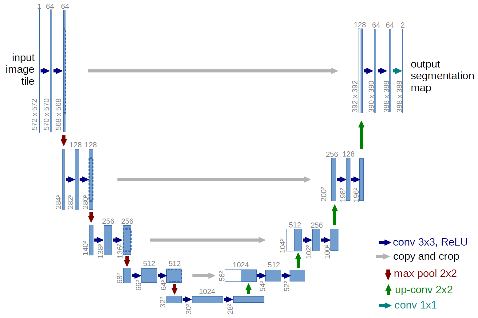 UNet architecture diagram.
1
2
3
4
5
6
7
8
9
10
11
12
13
14
15
16
17
18
19
20
21
22
23
24
25
26
27
28
29
30
31
32
33
34
35
36
37
38
39
40
41
42
43
44
45
46
47
48
49
50
51
52
53
54
55
56
57
58
59
60
61
62
63
64
65
66
def double_conv_block(x, n_filters):
    # Conv2D then ReLU activation
    x = layers.Conv2D(n_filters, 3, padding = "same", activation = "swish", kernel_initializer = "he_normal")(x) # relu act
    # Conv2D then ReLU activation
    x = layers.Conv2D(n_filters, 3, padding = "same", activation = "swish", kernel_initializer = "he_normal")(x) # relu act

    return x

def downsample_block(x, n_filters):
    f = double_conv_block(x, n_filters)
    p = layers.MaxPool2D(2)(f)
    p = layers.Dropout(0.1)(p)

    return f, p

def upsample_block(x, conv_features, n_filters):
    # upsample
    x = layers.Conv2DTranspose(n_filters,3, 2, activation = "relu", padding="same")(x)
    # concatenate
    x = layers.concatenate([x, conv_features])
    # dropout
    x = layers.Dropout(0.1)(x)
    # Conv2D twice with ReLU activation
    x = double_conv_block(x, n_filters)

    return x


def build_unet_model(img_shape=None):
    """ Builds a U-Net accepting 64x64 grayscale images by default
    """

    img_shape = (64,64,1) if not img_shape else img_shape
    # inputs
    inputs = layers.Input(shape=img_shape)

    # encoder: contracting path - downsample
    # 1 - downsample
    f1, p1 = downsample_block(inputs, 64)
    # 2 - downsample
    f2, p2 = downsample_block(p1, 128)
    # 3 - downsample
    f3, p3 = downsample_block(p2, 256)
    # 4 - downsample
    f4, p4 = downsample_block(p3, 512)

    # 5 - bottleneck
    bottleneck = double_conv_block(p4, 1024)

    # decoder: expanding path - upsample
    # 6 - upsample
    u6 = upsample_block(bottleneck, f4, 512)
    # 7 - upsample
    u7 = upsample_block(u6, f3, 256)
    # 8 - upsample
    u8 = upsample_block(u7, f2, 128)
    # 9 - upsample
    u9 = upsample_block(u8, f1, 64)

    # outputs
    outputs = layers.Conv2D(1, 1, padding="same", activation = "linear")(u9)

    # unet model with Keras Functional API
    unet_model = tf.keras.Model(inputs, outputs, name="U-Net")

    return unet_model
Our single image will be the famous “Lena” photo in one single channel (i.e. black and white). Let’s download it from Wikipedia :
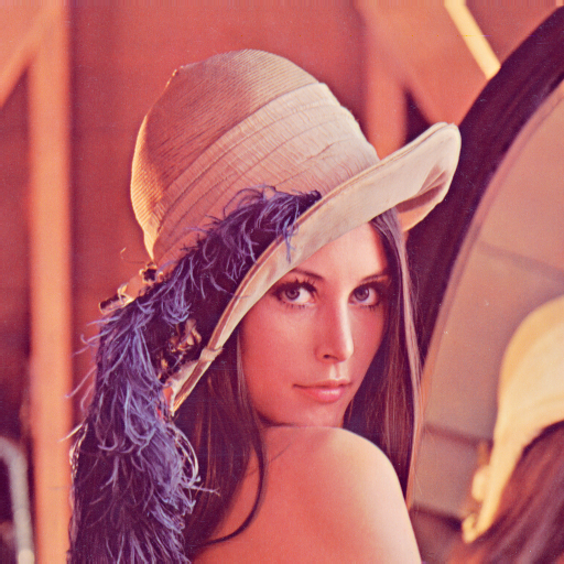 Lena photo.
1
!wget https://upload.wikimedia.org/wikipedia/en/7/7d/Lenna_%28test_image%29.png -O lena.png
1
2
3
# Load the image
lena_img = Image.open('lena.png').resize((64, 64)).convert('L')
lena_img

The method assumes all input image values lie in $[-1, 1]$
1
2
# Normalize the image so the values of its pixels lie between [-1, 1]
lena = (lena.astype(float) / 255.) * 2 - 1
Now we can create arrays with our fixed $\beta_t$ coefficients (and its $\alpha$ and $\bar\alpha_t$ derivations).
1
2
3
4
5
6
7
8
betas = np.linspace(1e-4, 0.04, num=300)  # linear increase schedule
alphas = 1 - betas
alphas_bars = np.cumprod(alphas)

# Also keep tensor copies
betas_tf = tf.convert_to_tensor(betas)
alphas_tf = tf.convert_to_tensor(alphas)
alphas_bars_tf = tf.convert_to_tensor(alphas_bars)
Let’s create the diffusion process, $q$.
1
2
3
4
5
6
7
8
9
10
11
12
13
14
15
16
17
18
19
20
21
22
23
24
25
26
27
28
29
30
31
32
33
34
35
def q(x0, t, return_noise=False):
    """ Gets a noised version of x0 sampling from q at time t

    Parameters
    ----------
        x0 : np.ndarray
            Initial image
        t : int
            timestep
        return_noise : bool
            Whether to also return the epsilon noise added

    Returns
    ----------
        Noised version of x0 at timestep t
    """
    if t == 0:
        return x0

    x0 = tf.cast(x0, tf.float32)

    mean = tf.cast(tf.sqrt(alpha_bar), tf.float32) * x0,
    var = tf.cast((1-alpha_bar), tf.float32)

    eps = tf.random.normal(
        shape=x0.shape
    )

    noised =  mean + tf.sqrt(var) * eps

    if not return_noise:
        return noised
    else:
        return noised, eps
The following image depicts an example of sampling from $q$ at several different timesteps:
 Diffusion process example.
Actually build the net
1
2
net = build_unet_model()
net.compile(optimizer='adam', loss='mse')
Define the dataloader, which will sample a random $x_t$ image and return (X, y) tuples with $(x_{t+1}, \epsilon)$.
1
2
3
4
5
6
7
8
9
10
11
12
13
14
15
16
17
18
19
20
21
22
23
24
BATCH_SIZE = 64
shape = (64,64)
x_0 = tf.cast(q(lena, 0), tf.float64)

def data_generator():
    for i in range(1024):
        # Get a random timestep
        t = tf.random.uniform(shape=(), minval=1, maxval=len(betas)-1, dtype=tf.int32)

        # Sample x_{t+1} and also get the noise epsilon that was added to it
        q_1, noise = q(lena, t, return_noise=True)

        # Ensure all shapes are correct
        q_1 = tf.reshape(q_1, shape)
        noise = tf.reshape(noise, shape)

        yield q_1, noise

# Build dataset from the above generator
dataset = tf.data.Dataset.from_generator(
    data_generator,
    output_signature = (tf.TensorSpec(shape=shape, dtype=tf.float32),
                        tf.TensorSpec(shape=shape, dtype=tf.float32))
).batch(BATCH_SIZE).prefetch(2)
Now, we’re able to train the model.
1
hist = net.fit(dataset, epochs=400)
Now we need to implement an inference function which accepts random noise (or any image) and let the process use our model for running the reverse diffusion part.
1
2
3
4
5
6
7
8
9
10
11
12
13
14
15
16
17
18
19
20
21
22
23
24
25
26
27
28
def inference(x, steps=len(betas)):
    # Save steps for plotting them later
    iterations = [x]

    for s in range(steps):
        t = steps - s

        beta = betas[t]
        alpha = alphas[t]
        alpha_bar = alphas_bars[t]

        # Predict added noise using our trained model
        eps = tf.squeeze(
            net(tf.reshape(iterations[-1], (1,64,64,1)))
        )

        # Get x_{t-1} (algorithm 2)
        mu =  tf.squeeze(
            (1 / alpha)  * ( iterations[-1]  - (beta / np.sqrt(1 - alpha_bar)) * eps)
        )

        z = tf.random.normal(shape=mu.shape) if t > 1 else 0

        new_img = mu + (z * np.sqrt(beta))

        iterations.append(new_img)

    return iterations
Okay, with all implemented, let’s start from a very noisy image and see whether it denoises it right
1
2
3
from_step = 180
plt.imshow(1 - q(lena, from_step).numpy().squeeze(), cmap='Greys',  interpolation='nearest')
plt.axis('off')

Run inference
1
2
3
4
results = inference(
    q(lena, from_step).numpy(),
    steps=from_step
)
Next figure shows an animation (concatenated images in results) of the inference process:

Improvements and further research
Since the publication of the paper several steps forward have been made.
One drawback of the method explained above is the way inference process works, as sampling one step at a time is clearly a bottleneck. With the intention of mitigating issue this, works like Song et al. 2021, Denoising Diffusion Implicit Models propose tricks aimed at improving inference speed.
Another interesting improvement is having more control on the generation process. For example, we could be only interested in generating dog pictures. An quite cool contribution on this is GLIDE, where a transformer is used for encoding a query text (e.g. “a dog”) and then combining that text representation with the internal U-Net activations. This way the image generation process becomes conditioned on what the user specifies via text, gaining more control.
Interesting resources
Here I link several extra resources I found very useful when learning about diffusion models (just in case you want to go down the rabbit hole).
[1] What are diffusion models?
[2] Ho et al (2020). “Denoising Diffusion Probabilistic Models”. The original paper.
[3] Ramesh et al (2022). DALL-E 2 paper.
[4] Imagen, the DALL-E 2 competitor from Google Brain, explained
Hope you’ve learned something new today!