Latent Consistency Models: How to speedup image generation

In a previous post I briefly covered Diffusion Models. And as I pointed out, they have an important drawback that makes them slow at creating new images. We often have to wait minutes for an image to be generated (even with beefy machines!). I’m talking about the “denoising” steps they have to run for generating an image.

–Denoising steps of a Diffusion Model to produce an image–

Reducing the generation latency is one of the key problems that have to be solved for this kind of model to become ubiquitous.

Recently, a very interesting tool came to the mainstream scene: krea.ai. It has a very interesting set of features that I consider steps forward towards the ideal way we’ll interact with diffusion models. Namely, one of the most interesting is its inference speed in the generation process, making it almost real time. See a quick demo of what I’m talking:

How is this even possible?. Well. One of the key techniques that makes these generations run as fast are the so called “Latent Consistency Models”, which come from this paper: Song et al. 2023. That’s what I’m covering in this post.

What is a Consistency Model?

(Diclaimer: I will take some mathematical licenses so this post is more legible for a profane reader. If you feel you need more rigorous or detailed explanations, I do refer you to the original paper.)

A consistency model is simply a model that tries to predict the initial state of a “Probability Flow”. If you recall the Diffusion Models post, I talked about an iterative “noising/denoising” process applied to an initial image. This “noising/denoising” is made by sampling random noise at each step and adding it to the image. This is the “Probability Flow” – the conjunction of all noise probability distributions at each step.

So, as I said above, a Consistency Model tries to approximate ODEs (Ordinary Differential Equations) that takes us from any point in de “noising chain” back to the beginning of it. I think this image is worth a thousand words:

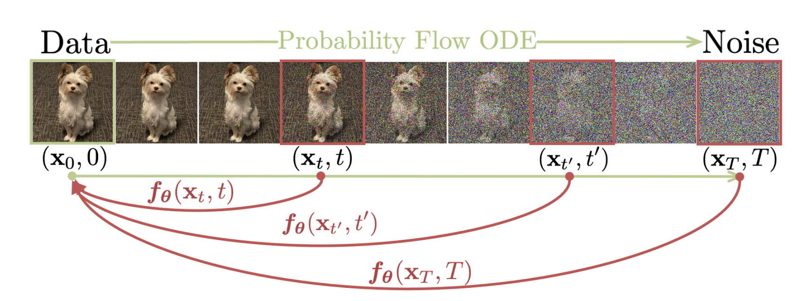
So, as you can see in the top part of the image we have an ODE that describes the change the image follows over time until it reaches the “pure noise state” (the “Probability Flow ODE arrow”). On the other hand, at the bottom, we have red arrows representing the “deinoising” ODEs from each point on the chain to the beginning (the “noiseless image”). As you see, the function that model this ODEs have a $\theta$ subscript, pointing us that they’ll be characterized by some kind of model.

In other words, this model will take an image at a point $T$ and will yield the original image, no matter how big is $T$.

Do you see the improvement? With this we could generate images in one run – much faster!

---

Important note: Consistency models act on the Pixel space (i.e, the original images). However, most of the Diffusion Models which are SOTA, work on the embedding (latent space). So, the Latent Consistency Models [ Luo et al. 2023] operate on the embedding space in which diffusion is applied (in models like Stable Diffusion) rather than on the image space (which is the classical space), but the idea is almost the same.

---

(Fun fact: They’re called Consistency Models as their output should be consistent with different $T$s; i.e. on the same trajectory*).

How do they work?

Supposing we have a well trained consistency model $f_{\theta}(x, T)$, we’ll be able to pass it a random noise image ($\hat{x}_T$) and some timestep $T$ in the chain (which we don’t necessarily have to know, as with the regular Diffusion Process) and it will instantly yield us the $\hat{x}_0$ image (i.e. the final generation) using a single forward run. Mathematically:

\[\begin{align*} \hat{x}_T \sim \mathcal{N}(0, I); \\ \hat{x}_0 = f_{\theta}(\hat{x}_T, T) \end{align*}\]

It’s worth pointing out, however, that this $f_\theta$ model can have errors (and sometimes it cannot have enough information for estimating the initial state). So the authors suggest that it can also be used multiple times. That is: denoising for a few steps (for example: 10) using the Consistency Model, run another few steps using the regular diffusion denoising procedure, run the Consistency model again… and so on. Or also applying this consistency model several times on different $T$’s

How are they trained?

There are two ways of training Consistency Models: 1) Consistency Distillation and 2) Model in Isolation

1. Training Consistency Models via Distillation

Oversimplifying, the way this works is:

1. Pick an image $x_0$ from the dataset.
2. Generate its “trajectory” towards the pure noise ($x_{0..T}$)
3. Use a numerical ODE solver (such as Euler or Heun) to calculate the ODE between pairs of points $(\hat{x_t}, x_{t+1})$. (Here $\hat{x}$ denotes the denoised image produced by a pretrained diffusion model)
4. Fit the $f_{\theta}$ consistency model with those pair of points and the Consistency Distillation Loss (or $\mathcal{L}^{N}_{CD}$)

\[\begin{align*} \mathcal{L}^{N}_{CD}(\theta, \theta^{-}, \phi) = \mathbb{E}[\lambda(t_n) d(f_\theta(x_{t+1}, t_{n+1}), f_{\theta^-}(x_{t}, t_{n}) ) ] \end{align*}\]

The above function seems quite verbose, but let’s take a look at each one of the terms:

• $\theta^{-}$: is just a running average of the previous weights of the model and it’s not optimized.
• $\phi$: The “denoiser” model (aka. the diffusion model)
• $\lambda$: Is just a weighting function. Actually, researchers fix it to 1 always.
• $d$: Is a metric function defined in the range [0, $\infty$) and measures how similar the two samples are (0 = equal, infinite=totally different). Just for reference, functions that satisfy this requirement are the L2 and L1 distances.

2. Training Consistency Models via Model in Isolation

This “training mode” is presented with the idea of not having to rely in a pretrained diffusion model which estimates $\nabla\log p_t(x_t)$.

With some mathematical magic (proofs are in the appendix), they can replace the prediction of the diffusion model with the following expression:

\[\begin{align*} \nabla\log p_t(x_t) \approx \frac{-x_t - x}{t^2} \end{align*}\]

where $p_t$ is the probabilty flow for going backwards in the chain.

Results

Here I share some of the results of the technique, but from the Latent Consistency Models paper, which is what’s actually used on all the big generative models:

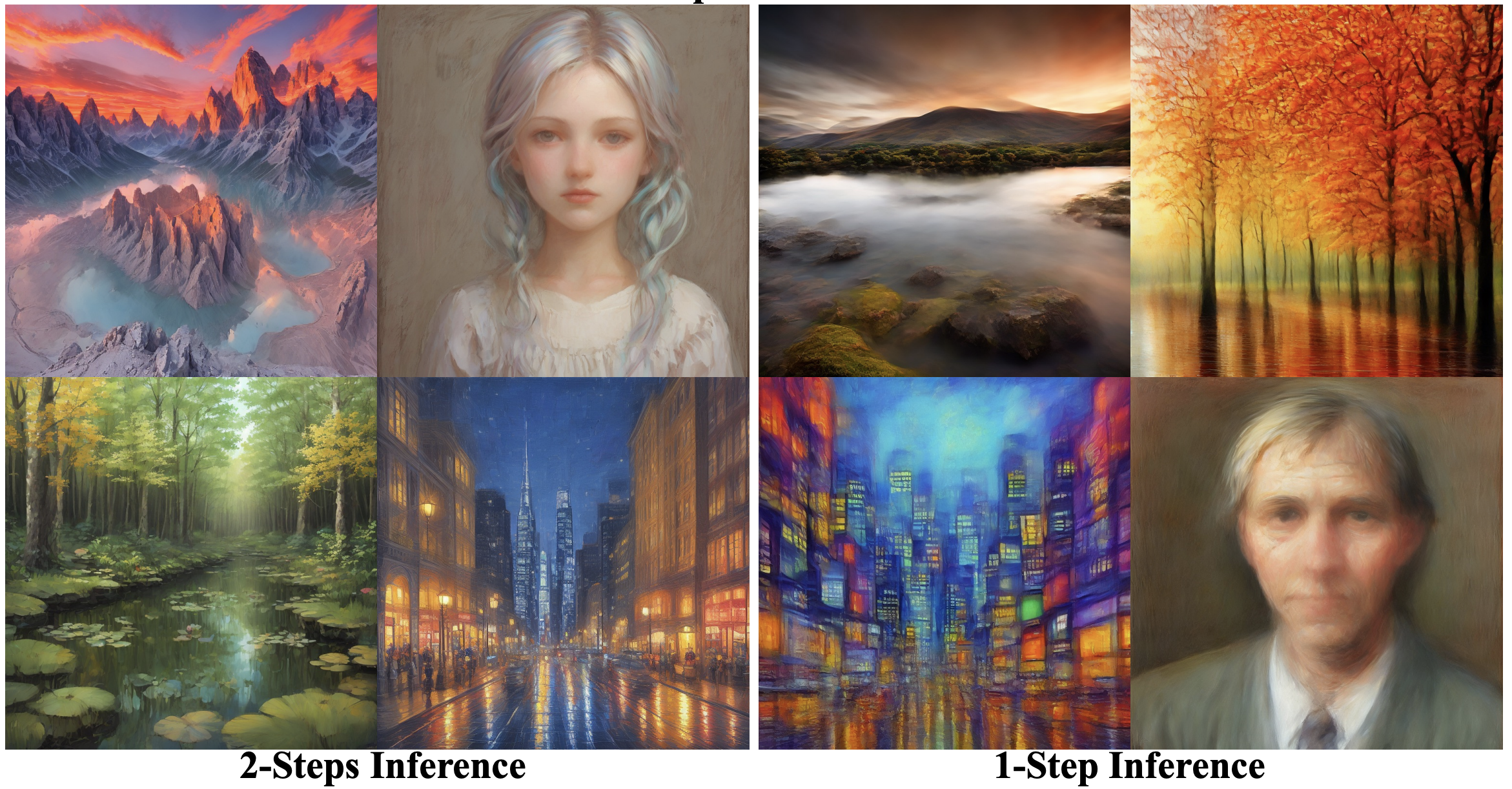
Just after being trained, with a few steps, we can generate images of impressive quality!

Playing with it

Recently, a HuggingFace space has been created for demonstrating how image generation is instantly done with this technique. You can play with it here! https://huggingface.co/spaces/ilumine-AI/LCM-Painter

I also recorded one of the interactions I made with it. All of it is real time! 🤯

Closing up

In this post I briefly covered Consistency Models, which is a very clever idea that dramatically improves the quality of the interactions we have with image generation models. This is the kind of contributions that will redefine the future on how we’ll work with them!

(29/11/2023: Edit post writing)

Stability.ai just published SDXL-turbo which is a version of Stable Diffusion that runs in nearly real time with very good results (even improving LCM’s).

The main advancement behind this achievement has been the introduction of a new method called Adversarial Diffusion Distillation. Worth checking it out!